
Conditional Formatting Rules Manager Screenshot

Conditional Formatting Menu Screenshot

Conditional Formatting Screenshot - Stop If True

Conditional Formatting Show For Sheet Screenshot

Conditional Formatting Duplicate Values Rule Screenshot

Conditional Formatting Custom Formula Rule Screenshot

Track Active Cell VBA Code
- Click Alt+F11 to open the Visual Basic Editor.
- Find this workbook in the top-left window, and expand it to find this worksheet and double-click it.
- In the worksheet you want to track the active cell in, paste the code. Note that you will have to repeat this step unless you save the file as a macro-enabled file (.xlsm).
Private Sub Worksheet_SelectionChange(ByVal Target As Range)
ActiveCell.Calculate
End Sub
Conditional Formatting Consolidated Tie-out Sheet Screenshot

 Overview
Conditional Formatting is one of the most powerful features in Excel, yet people don’t seem to use it near enough. So many things can be automated in Excel, and this is certainly no exception. From finding the risk in your data to giving it a polished look, there are dozens of built-in options to use. In this article, we’ll discuss the what, why, and how of conditional formatting, followed up by some gotchas, tips, tricks, examples, and macros that make it super-easy to use. Make sure to download the accompanying workbook that contains several examples you can copy and learn from!
 What is conditional formatting
Conditional formatting is exactly what it sounds like – the ability to apply formatting based on certain conditions. Here are some details:
- You can specify the ranges to apply your conditional formatting to, including single cells, multiple cells, rows, and columns.
- There are several built-in options like icons, color scales, and data bars that help you visually understand your data.
- Multiple rules can be applied to the same range in a prioritized manner with the lower-listed rules taking precedence.
- Conditional formatting overrides fixed formatting.
- The most powerful and flexible option is defining a custom formula.
 Why should conditional formatting be used?
There are several benefits to using conditional formatting:
- It automates the formatting, so as your data changes or grows, the formats can update dynamically.
- It allows you to address risks, such as differences, errors, blanks, and unwanted hard-coded values.
- It allows you to quickly compare data, such as the top few and bottom few values.
- It adds clarity to your data, making it easier to communicate to key stakeholders.
- It gives your data a professional look with precise colors, borders, and number formats.
 How do you use conditional formatting?
Conditional formatting is applied primarily using the conditional formatting rules manager 🖼️, located on the Home tab 🖼️ in the ribbon. This box is powerful and has several pre-set options you can quickly apply, such as cells matching a value, top/bottom values, or unique/duplicate values. The most flexible option is defining your own formula for the conditions that drive your desired formats. Once you determine the conditions and formats you want to use, follow these three steps to apply conditional formatting:
- Select the range you want to apply the conditional formatting rules to. You can also adjust this afterwards if you need to.
- Determine the conditions. For custom conditions, enter the formula in a boolean style, for example =A2=”Gold” or =A2>50 without the IF at the beginning. For multiple conditions, wrap them in AND, OR, or both, remembering your order of operations. Be careful to use the correct absolute or relative references in any custom formulas. Start simple if using custom formulas!
- Determine the formatting you want to use. Most (but not all) formats are available. For example, alignment is not an option you can conditionally format.
See the Macros section below for a couple of even easier ways to apply conditional formatting!
 Gotchas
Be aware of several gotchas related to conditional formatting:
Make sure you name ranges uniquely, logically, and consistently.
- Conditional formatting overrides fixed formatting. If you’re tearing your hair out trying to format cells and it doesn’t seem to work, check out any conditional formatting rules that might be applied for your selected range.
- Conditional formatting rules are applied in a prioritized fashion and can conflict with one another. If they aren’t working how you’d expect, review the priority and adjust if needed.
- Sometimes the ranges can get messed up due to Excel bugs, both in custom formula conditions and the range to apply to. Adjust them once and they should be fine.
- When cutting, copying, and pasting, conditional formatting will generally follow along. This can create unintended issues and inconsistent formatting, so review the conditional formatting rules before and after in the range you’re pasting to.
- In general, it’s good to not overuse formatting so it doesn’t become distracting. This is especially important with conditional formatting because of the calculations required – overuse can cause performance to slow down considerably!
 Tips & tricks
- To review all the conditional rules in the entire sheet, toggle the option 🖼️ in the rules manager to see them all and how they’re prioritized.
- To help prevent conflicting rules, you can use the “Stop if true” 🖼️ option for your conditional formatting rules. This will skip all other rules that apply to the same cells.
- Stop if true 🖼️ is also a great way to PAUSE conditional formatting rules. This is often helpful for reviewing drafts, then turning them back on when finished. See the Conditional Formatting Picker macro below for an awesome shortcut!
- Conditional formatting is great for checks – comparing amounts, indicating status, etc. I like to consolidate all of these checks in one sheet 🖼️ for easy reference.
- Colors are the most common way to use conditional formatting. Use them consistently and consider that some users might be colorblind, so have an alternate way to evaluate your data.
 Examples
Below are several helpful conditional formatting examples worth considering. To get a copy of these examples, use the form at the top or bottom to get a helpful workbook! The XLEV8 Excel Add-in allows you to apply these conditional formats in one step with shortcuts.
 |
Heat scale Shades cells based on relative values. Good for shading several different values in a column, row, or both. How to add: select the range to format, then use the Color Scales option on the Conditional Formatting menu 🖼️. |
 |
Data bars Shows in-cell horizontal bars based on relative values. Good for comparing several values in a column. How to add: select the range to format, then use the Data Bars option on the Conditional Formatting menu 🖼️. |
 |
Icons Shows one of three different icons (several icon set options) based on three relative groupings from the data set values. How to add: select the range to format, then use the Icon Sets option on the Conditional Formatting menu 🖼️. |
 |
Top/bottom values Formats cells containing the top/bottom n values or percentages among the selected data set. For example, format the top 5 salespeople in a month. How to add: select the range to evaluate, then use the Top/Bottom Rules option on the Conditional Formatting menu 🖼️. |
 |
Find Duplicates Formats cells appearing more than once in the selected data set. You can also take a similar approach to highlight unique values. How to add: select the range to evaluate, then in the Conditional Formatting Rules Manager, add a new rule and select the format only unique or duplicate values option 🖼️. |
 |
Find Blanks Formats blank cells within the data set How to add: select the range to evaluate, then in the Conditional Formatting Rules Manager, add a new rule and select the use a formula to determine which cells to format option 🖼️. Then enter this formula (changing the cell reference to meet your needs): =B12=”” |
 |
Find Differences Formats cells that have different values between two ranges of the same size. How to add: select the range that is being compared, then in the Conditional Formatting Rules Manager, add a new rule and select the use a formula to determine which cells to format option 🖼️. Then enter this formula (changing the cell references to meet your needs): =C12<>B12 |
 |
Find Errors Formats cells within your data set that contain formulas resulting in an error (i.e. #NAME? or #N/A). How to add: select the range to evaluate, then in the Conditional Formatting Rules Manager, add a new rule and select the use a formula to determine which cells to format option 🖼️. Then enter this formula (changing the cell references to meet your needs): =ISERROR(B12)=TRUE |
 |
Tie-outs Formats cells with a pre-defined good or bad format based on whether the cell value is within a threshold (generally zero). Often used for comparing or tying-out financial figures. How to add: select the range to evaluate, then in the Conditional Formatting Rules Manager, add two new rules and select the use a formula to determine which cells to format option 🖼️. Then enter these formulas (changing the cell references and comparisons to meet your needs): =ROUND(B12,2)<>0 =ROUND(B12,2)=0 |
 |
Find Hard-Coded Values Formats cells containing hard-coded values (not the result of formulas). This is useful for addressing the risk that numbers were manipulated within your data set. How to add: select the range to evaluate, then in the Conditional Formatting Rules Manager, add a new rule and select the use a formula to determine which cells to format option 🖼️. Then enter this formula (changing the cell references to meet your needs): =AND(ISBLANK(B12)=FALSE,ISFORMULA(B12)= FALSE,ISTEXT(B12)=FALSE) |
 |
Find Hard-Coded Formula Values Formats cells containing formulas with hard-coded value components. This is useful for addressing the risk that numbers were manipulated within your data set. How to add: this requires the use of a user-defined function that can determine if hard-coded values appear in the formula. Select the range to evaluate, then use the Conditional Formatting Picker (option F) in the XLEV8 Excel Add-in to apply this conditional format |
 |
Row Banding Shades rows with alternating colors, which often helps read them more clearly. How to add: select the range to format, then in the Conditional Formatting Rules Manager, add a new rule and select the use a formula to determine which cells to format option 🖼️. Then enter these formulas (changing the cell references and comparisons to meet your needs): =MOD(SUBTOTAL(3,$B$11:$B12),2)=0 =MOD(SUBTOTAL(3,$B$11:$B12),2)=1 |
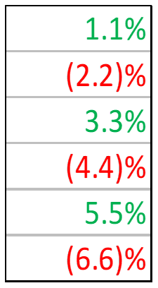 |
Variances Formats variance amounts +/- zero. How to add: select the range to format, then in the Conditional Formatting Rules Manager, add a new rule and select the use a formula to determine which cells to format option 🖼️. Then enter these formulas (changing the cell references and comparisons to meet your needs): =AND(B12<>”N/A”,B12<0) =AND(B12<>”N/A”,B12>0) |
 |
Find Values Formats cells with matching partial or full values. How to add: select the range to format, then in the Conditional Formatting Rules Manager, add a new rule and select the use a formula to determine which cells to format option 🖼️. Then enter this formula (changing the cell references and comparisons to meet your needs): =SEARCH(“dog”,$B1)>0 |
 |
Find Text Lengths Formats cells with certain text lengths (using equals, does not equal, greater than, less than, etc.). How to add: select the range to format, then in the Conditional Formatting Rules Manager, add a new rule and select the use a formula to determine which cells to format option 🖼️. Then enter this formula (changing the cell references and comparisons to meet your needs): =LEN(B12)>=7 |
 |
Track Active Cell/Column/Row Formats the active cell, column, or row based on what you have selected. How to add: to track your active cell as you select different cells, this requires adding VBA code 🖼️ to the worksheet. To add the conditional formatting, select the range to format, then in the Conditional Formatting Rules Manager, add two new rules and select the use a formula to determine which cells to format option 🖼️. Then enter these formulas (changing the cell references and comparisons to meet your needs) to track the active cell, row, and column: =AND(COLUMN()=CELL(“COL”),ROW()= CELL(“ROW”)) =ROW()=CELL(“ROW”) =COLUMN()=CELL(“COL”) |
 Macros That Help
There are two valuable macros in the XLEV8 Excel Add-in that can automate applying conditional formatting and provide shortcuts:
- Conditional Formatting Picker – this offers shortcuts to several conditional formatting types in one picklist, including the examples above, as well as the ability to pause rules, clear rules, and jump to the rules manager.
- Bulk Conditional Formats – this lets you apply several conditional formatting rules in one bulk step. If you have very specific rules and formats you like to use, this makes it very quick and easy to reuse them!
 Summary
If you want to make your Excel files look awesome with polished, dynamic formatting, conditional formatting is an awesome tool. It’s also extremely helpful for visually analyzing your data and identifying errors, exceptions, and extremes in your data. Hopefully this article got you thinking about several ways you can leverage conditional formatting. I use it in almost every Excel file, from complex models to basic to-do lists, and the macros above help use them with extreme efficiency! Make sure to grab a copy of the template using the form above to get several helpful conditional formatting examples you can use!
How have you leveraged conditional formatting to make your Excel files quicker and more effective? Let us know in the comments below!


Recent Comments